How to control and understand settings in the Format Cells dialog box in Excel
Summary
Microsoft Excel lets you change many of the ways it displays data in a cell. For example, you can specify the number of digits to the right of a decimal point, or you can add a pattern and border to the cell. You can access and modify the majority of these settings in the Format Cells dialog box (on the Format menu, click Cells).
The «More Information» section of this article provides information about each of the settings available in the Format Cells dialog box and how each of these settings can affect the way your data is presented.
More Information
There are six tabs in the Format Cells dialog box: Number, Alignment, Font, Border, Patterns, and Protection. The following sections describe the settings available in each tab.
Number Tab
Auto Number Formatting
By default, all worksheet cells are formatted with the General number format. With the General format, anything you type into the cell is usually left as-is. For example, if you type 36526 into a cell and then press ENTER, the cell contents are displayed as 36526. This is because the cell remains in the General number format. However, if you first format the cell as a date (for example, d/d/yyyy) and then type the number 36526, the cell displays 1/1/2000.
There are also other situations where Excel leaves the number format as General, but the cell contents are not displayed exactly as they were typed. For example, if you have a narrow column and you type a long string of digits like 123456789, the cell might instead display something like 1.2E+08. If you check the number format in this situation, it remains as General.
Finally, there are scenarios where Excel may automatically change the number format from General to something else, based on the characters that you typed into the cell. This feature saves you from having to manually make the easily recognized number format changes. The following table outlines a few examples where this can occur:
| If you type | Excel automatically assigns this number format |
|---|---|
| 1.0 | General |
| 1.123 | General |
| 1.1% | 0.00% |
| 1.1E+2 | 0.00E+00 |
| 1 1/2 | # ?/? |
| $1.11 | Currency, 2 decimal places |
| 1/1/01 | Date |
| 1:10 | Time |
Generally speaking, Excel applies automatic number formatting whenever you type the following types of data into a cell:
Built-in Number Formats
Excel has a large array of built-in number formats from which you can choose. To use one of these formats, click any one of the categories below General and then select the option that you want for that format. When you select a format from the list, Excel automatically displays an example of the output in the Sample box on the Number tab. For example, if you type 1.23 in the cell and you select Number in the category list, with three decimal places, the number 1.230 is displayed in the cell.
These built-in number formats actually use a predefined combination of the symbols listed below in the «Custom Number Formats» section. However, the underlying custom number format is transparent to you.
The following table lists all of the available built-in number formats:
| Number format | Notes |
|---|---|
| Number | Options include: the number of decimal places, whether or not the thousands separator is used, and the format to be used for negative numbers. |
| Currency | Options include: the number of decimal places, the symbol used for the currency, and the format to be used for negative numbers. This format is used for general monetary values. |
| Accounting | Options include: the number of decimal places, and the symbol used for the currency. This format lines up the currency symbols and decimal points in a column of data. |
| Date | Select the style of the date from the Type list box. |
| Time | Select the style of the time from the Type list box. |
| Percentage | Multiplies the existing cell value by 100 and displays the result with a percent symbol. If you format the cell first and then type the number, only numbers between 0 and 1 are multiplied by 100. The only option is the number of decimal places. |
| Fraction | Select the style of the fraction from the Type list box. If you do not format the cell as a fraction before typing the value, you may have to type a zero or space before the fractional part. For example, if the cell is formatted as General and you type 1/4 in the cell, Excel treats this as a date. To type it as a fraction, type 0 1/4 in the cell. |
| Scientific | The only option is the number of decimal places. |
| Text | Cells formatted as text will treat anything typed into the cell as text, including numbers. |
| Special | Select one of the following from the Type box: Zip Code, Zip Code + 4, Phone Number, and Social Security Number. |
Custom Number Formats
If one of the built-in number formats does not display the data in the format that you require, you can create your own custom number format. You can create these custom number formats by modifying the built-in formats or by combining the formatting symbols into your own combination.
Before you create your own custom number format, you need to be aware of a few simple rules governing the syntax for number formats:
Each format that you create can have up to three sections for numbers and a fourth section for text.
The first section is the format for positive numbers, the second for negative numbers, and the third for zero values.
These sections are separated by semicolons.
If you have only one section, all numbers (positive, negative, and zero) are formatted with that format.
You can prevent any of the number types (positive, negative, zero) from being displayed by not typing symbols in the corresponding section. For example, the following number format prevents any negative or zero values from being displayed:
To set the color for any section in the custom format, type the name of the color in brackets in the section. For example, the following number format formats positive numbers blue and negative numbers red:
Instead of the default positive, negative and zero sections in the format, you can specify custom criteria that must be met for each section. The conditional statements that you specify must be contained within brackets. For example, the following number format formats all numbers greater than 100 as green, all numbers less than or equal to -100 as yellow, and all other numbers as cyan:
Apply or remove cell borders on a worksheet
By using predefined border styles, you can quickly add a border around cells or ranges of cells. If predefined cell borders do not meet your needs, you can create a custom border.
Note: Cell borders that you apply appear on printed pages. If you do not use cell borders but want worksheet gridline borders to be visible on printed pages, you can display the gridlines. For more information, see Print with or without cell gridlines.
On a worksheet, select the cell or range of cells that you want to add a border to, change the border style on, or remove a border from.
On the Home tab, in the Font group, do one of the following:
To apply a new or different border style, click the arrow next to Borders  , and then click a border style.
Tip: To apply a custom border style or a diagonal border, click More Borders. In the Format Cells dialog box, on the Border tab, under Line and Color, click the line style and color that you want. Under Presets and Border, click one or more buttons to indicate the border placement. Two diagonal border buttons 
 are available under Border.
To remove cell borders, click the arrow next to Borders , and then click No Border .
The Borders button displays the most recently used border style. You can click the Borders button (not the arrow) to apply that style.
If you apply a border to a selected cell, the border is also applied to adjacent cells that share a bordered cell boundary. For example, if you apply a box border to enclose the range B1:C5, the cells D1:D5 acquire a left border.
If you apply two different types of borders to a shared cell boundary, the most recently applied border is displayed.
A selected range of cells is formatted as a single block of cells. If you apply a right border to the range of cells B1:C5, the border is displayed only on the right edge of the cells C1:C5.
If you want to print the same border on cells that are separated by a page break, but the border appears on only one page, you can apply an inside border. This way, you can print a border at the bottom of the last row of one page and use the same border at the top of the first row on the next page. Do the following:
Select the rows on both sides of the page break.
Click the arrow next to Borders , and then click More Borders.
Under Presets, click the Inside button  .
.
Under Border, in the preview diagram, remove the vertical border by clicking it.
On a worksheet, select the cell or range of cells that you want to remove a border from.
To cancel a selection of cells, click any cell on the worksheet.
On the Home tab, in the Font group, click the arrow next to Borders , and then click No Border .
Click Home > the Borders arrow > Erase Border, and then select the cells with the border you want to erase.
You can create a cell style that includes a custom border, and then you can apply that cell style when you want to display the custom border around selected cells.
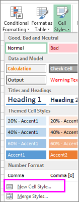
On the Home tab, in the Styles group, click Cell Styles.
Tip: If you do not see the Cell Styles button, click Styles, and then click the More button next to the cell styles box.
Click New Cell Style.
In the Style name box, type an appropriate name for the new cell style.
On the Border tab, under Line, in the Style box, click the line style that you want to use for the border.
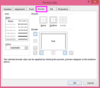
In the Color box, select the color that you want to use.
Under Border, click the border buttons to create the border that you want to use.
In the Style dialog box, under Style Includes (By Example), clear the check boxes for any formatting that you do not want to include in the cell style.
To apply the cell style, do the following:
Select the cells that you want to format with the custom cell border.
On the Home tab, in the Styles group, click Cell Styles.
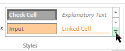
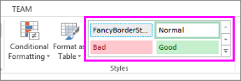
Click the custom cell style that you just created. Like the FancyBorderStyle button in this picture.
To customize the line style or color of cell borders or erase existing borders, you can use the Draw Borders options. To draw cell borders, you’ll first select the border type, then the border color and line style, and select the cells that you want to add a border around. Here’s how:
Click Home > the Borders arrow  .
.
Pick Draw Borders for outer borders or Draw Border Grid for gridlines.
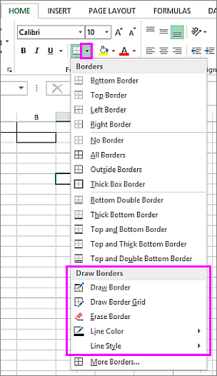
Click the Borders arrow > Line Color arrow, and then pick a color.
Click the Borders arrow > Line Style arrow, and then pick a line style.
Select cells you want to draw borders around.
Add a border, border color, or border line style
Select the cell or range of cells that you want to add a border around, change the border style on, or remove a border from.
2. Click Home > the Borders arrow, and then pick the border option you want.
Add a border color — Click the Borders arrow > Border Color, and then pick a color
Add a border line style — Click the Borders arrow > Border Style, and then pick a line style option.
The Borders button shows the most recently used border style. To apply that style, click the Borders button (not the arrow).
If you apply a border to a selected cell, the border is also applied to adjacent cells that share a bordered cell boundary. For example, if you apply a box border to enclose the range B1:C5, the cells D1:D5 will acquire a left border.
If you apply two different types of borders to a shared cell boundary, the most recently applied border is displayed.
A selected range of cells is formatted as a single block of cells. If you apply a right border to the range of cells B1:C5, the border is displayed only on the right edge of the cells C1:C5.
If you want to print the same border on cells that are separated by a page break, but the border appears on only one page, you can apply an inside border. This way, you can print a border at the bottom of the last row of one page and use the same border at the top of the first row on the next page. Do the following:
Select the rows on both sides of the page break.
Click the arrow next to Borders , and then click the Inside Horizontal Border
Remove a border
To remove a border, select the cells with the border and click the Borders arrow > No Border.
Need more help?
You can always ask an expert in the Excel Tech Community or get support in the Answers community.