Checking formatting in excel

How to control and understand settings in the Format Cells dialog box in Excel

Summary

Microsoft Excel lets you change many of the ways it displays data in a cell. For example, you can specify the number of digits to the right of a decimal point, or you can add a pattern and border to the cell. You can access and modify the majority of these settings in the Format Cells dialog box (on the Format menu, click Cells).

The «More Information» section of this article provides information about each of the settings available in the Format Cells dialog box and how each of these settings can affect the way your data is presented.

More Information

There are six tabs in the Format Cells dialog box: Number, Alignment, Font, Border, Patterns, and Protection. The following sections describe the settings available in each tab.

Number Tab

Auto Number Formatting

By default, all worksheet cells are formatted with the General number format. With the General format, anything you type into the cell is usually left as-is. For example, if you type 36526 into a cell and then press ENTER, the cell contents are displayed as 36526. This is because the cell remains in the General number format. However, if you first format the cell as a date (for example, d/d/yyyy) and then type the number 36526, the cell displays 1/1/2000.

There are also other situations where Excel leaves the number format as General, but the cell contents are not displayed exactly as they were typed. For example, if you have a narrow column and you type a long string of digits like 123456789, the cell might instead display something like 1.2E+08. If you check the number format in this situation, it remains as General.

Finally, there are scenarios where Excel may automatically change the number format from General to something else, based on the characters that you typed into the cell. This feature saves you from having to manually make the easily recognized number format changes. The following table outlines a few examples where this can occur:

If you type	Excel automatically assigns this number format
1.0	General
1.123	General
1.1%	0.00%
1.1E+2	0.00E+00
1 1/2	# ?/?
$1.11	Currency, 2 decimal places
1/1/01	Date
1:10	Time

Generally speaking, Excel applies automatic number formatting whenever you type the following types of data into a cell:

Built-in Number Formats

Excel has a large array of built-in number formats from which you can choose. To use one of these formats, click any one of the categories below General and then select the option that you want for that format. When you select a format from the list, Excel automatically displays an example of the output in the Sample box on the Number tab. For example, if you type 1.23 in the cell and you select Number in the category list, with three decimal places, the number 1.230 is displayed in the cell.

These built-in number formats actually use a predefined combination of the symbols listed below in the «Custom Number Formats» section. However, the underlying custom number format is transparent to you.

The following table lists all of the available built-in number formats:

Number format	Notes
Number	Options include: the number of decimal places, whether or not the thousands separator is used, and the format to be used for negative numbers.
Currency	Options include: the number of decimal places, the symbol used for the currency, and the format to be used for negative numbers. This format is used for general monetary values.
Accounting	Options include: the number of decimal places, and the symbol used for the currency. This format lines up the currency symbols and decimal points in a column of data.
Date	Select the style of the date from the Type list box.
Time	Select the style of the time from the Type list box.
Percentage	Multiplies the existing cell value by 100 and displays the result with a percent symbol. If you format the cell first and then type the number, only numbers between 0 and 1 are multiplied by 100. The only option is the number of decimal places.
Fraction	Select the style of the fraction from the Type list box. If you do not format the cell as a fraction before typing the value, you may have to type a zero or space before the fractional part. For example, if the cell is formatted as General and you type 1/4 in the cell, Excel treats this as a date. To type it as a fraction, type 0 1/4 in the cell.
Scientific	The only option is the number of decimal places.
Text	Cells formatted as text will treat anything typed into the cell as text, including numbers.
Special	Select one of the following from the Type box: Zip Code, Zip Code + 4, Phone Number, and Social Security Number.

Custom Number Formats

If one of the built-in number formats does not display the data in the format that you require, you can create your own custom number format. You can create these custom number formats by modifying the built-in formats or by combining the formatting symbols into your own combination.

Before you create your own custom number format, you need to be aware of a few simple rules governing the syntax for number formats:

Each format that you create can have up to three sections for numbers and a fourth section for text.

The first section is the format for positive numbers, the second for negative numbers, and the third for zero values.

These sections are separated by semicolons.

If you have only one section, all numbers (positive, negative, and zero) are formatted with that format.

You can prevent any of the number types (positive, negative, zero) from being displayed by not typing symbols in the corresponding section. For example, the following number format prevents any negative or zero values from being displayed:

To set the color for any section in the custom format, type the name of the color in brackets in the section. For example, the following number format formats positive numbers blue and negative numbers red:

Instead of the default positive, negative and zero sections in the format, you can specify custom criteria that must be met for each section. The conditional statements that you specify must be contained within brackets. For example, the following number format formats all numbers greater than 100 as green, all numbers less than or equal to -100 as yellow, and all other numbers as cyan:

Источник

How to See Formatting in Excel 2013

Microsoft Excel spreadsheets can have a lot of different types of formatting. Usually, Excel will be able to determine the appropriate formatting type based on the type of data you have entered, but this doesn’t always work correctly. if you suspect that there is a problem then you might be wondering how to see formatting in Excel.

How to Check a Cell’s Format in Excel 2013

1. Open the spreadsheet.
2. Select the cell.
3. Choose the Home tab.
4. Find the format type in the Number group dropdown menu.

Our guide continues below with additional information on how to see formatting in Excel, including pictures of these steps.

Different types of cell formats will display your data differently in Excel 2013. Changing the format of a cell to best suit the data contained within it is a simple way to ensure that your data displays correctly.

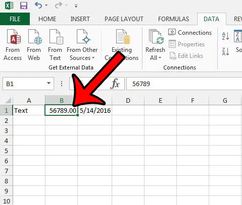
For example, a date that is formatted as a “Date” cell might display as “6/27/2016.” However, if that same cell is formatted as a number, then it might display as “42548.00” instead. This is just one example of why it is important to use proper formatting when possible.

If data is not displaying properly in a cell, then you should check the cell formatting before you start troubleshooting. Our guide below will show you a quick location to check so you can see the formatting that is currently applied to a cell.

If you are trying to fix error issues with the VLOOKUP formula, then our article on how to make n/a 0 in Excel can save you some headaches.

What Format is a Cell in My Spreadsheet? (Guide with Pictures)

This guide will show you how to select a cell, and then see the format of that cell. This is helpful information to have if you are having certain types of issues that are difficult to fix. For example, you might need to check a cell’s format if the cell contains a formula that is not updating. So continue reading below to see how to view the format currently applied to a cell.

Step 1: Open the spreadsheet in Excel 2013.

Step 2: Click the cell for which you wish to view the current format.

Step 3: Click the Home tab at the top of the window.

Step 4: Locate the drop-down menu at the top of the Number section in the ribbon.

The value shown in the drop-down is the current format for your cell. The format of the cell that is currently selected is “Number.” If you click that drop-down menu, you can select a different format for the currently-selected cell.

Now that you know how to see formatting in Excel you will be able to check for that information more easily so that you can make necessary changes. For example, you could convert text to numbers in Excel using that tool.

Our tutorial continues below with additional discussion about how to check the format on a cell in Excel.

More Information on How to View Formatting in Microsoft Excel

There are a lot of different formatting options that you can apply to some of the cells in your worksheet when you right-click on a cell and choose the Format Cells option. Some of the options that you will see on the Format Cells dialog box include:

• Currency format – if you are going to be working with monetary values then this can be preferable to using one of the number formatting options
• Number format – occasionally the “General” formatting option might not work properly if you are dealing with large number values, or if you copy and paste data from another source.
• Text format
• Percentage format
• Date format
• Time format
• Fraction format
• Scientific format – if you are going to be working with scientific notation or have multiple lines in a lot of your cells, then you might not see the options you need on the number tab in the ribbon, which can make this a more useful formatting selection.

There are more than that, and you also have the ability to see your own custom format if you are dealing with something like large numbers, or if your selected cells contain needs an uncommon registered trademarks symbol, or a currency symbol, that isn’t offered as a formatting choice by default.

Some of the formatting options are going to let you do things like adjust the number of decimal places if you need to increase decimal or decrease decimal content.

You can also find some of the more common formatting options if you choose the Home tab at the top of the window, then look at the different buttons in the Number group of the ribbon.

In addition to these formatting options there are also groups on the Home ribbon where you can do things like adjust the font color or font size, or switch the text alignment for your selected cells.

When you change the formatting for some of your cell data if can affect the way that it displays in the cells. This could lead to your columns not being wide enough to fit all of the data, so you might need to double-click on a column border to display everything if you are starting to see numeric values as scientific notation.

Do you want to remove all of the formatting from a cell and start from scratch? This article – https://www.solveyourtech.com/removing-cell-formatting-excel-2013/ – will show you a short method that clears all of the formatting from a cell.

Additional Sources

Matthew Burleigh has been writing tech tutorials since 2008. His writing has appeared on dozens of different websites and been read over 50 million times.

After receiving his Bachelor’s and Master’s degrees in Computer Science he spent several years working in IT management for small businesses. However, he now works full time writing content online and creating websites.

His main writing topics include iPhones, Microsoft Office, Google Apps, Android, and Photoshop, but he has also written about many other tech topics as well.

Источник

How to check date format in Excel

I have around 20,000 records in an Excel file and around four columns which have dates. I am trying to insert those into SQL. However date columns have dates in incorrect format eg; 02/092015 or 02/90/2015 or 2015 . So checking 20,000 records one by one would be very lengthy.

I tried to count / but it didn’t work. It changes the format of column to date.

I was looking for some formula which can check the format and maybe color the cell or something like it.

3 Answers 3

I was running across this issue today, and would like to add on to what nekomatic started.

Before we begin, the TEXT formula needs to follow the date format we are working with. If your dates are in month/day/year format, then your second argument for the TEXT formula would be «mm/dd/yyyy». If it is in the format day/month/year, then the formula would need to use «dd/mm/yyyy». For the purposes of my answer here, I am going to have my dates in month/day/year format.

Now, let’s assume that cell A1 contains the value 12/1/2015 , cell A2 contains the value monkey , and cell A3 contains the value 2015 . Further, let’s assume our minimum acceptable date is December 1st, 2000.

In column B, we will enter the formula

=IF(ISERROR(DATEVALUE(TEXT(A1,»mm/dd/yyyy»))),»not a date»,IF(A1 >=DATEVALUE(TEXT(«01/01/2000″,»mm/dd/yyyy»)),A1,»not a valid date»))

The above formula will validate correct dates, test against non-date values, incomplete dates, and date values outside of an acceptable minimal value.

Our results in column B should then show 12/1/2015 , not a date , and not a valid date .

Источник