Irr functions in excel

IRR function in Excel and the example how to count IRR

For calculating the internal rate of return (of the internal rate of return, IRR) in Excel the IRR function is used. Its features, syntax, examples we are discussed in this article.

The features and syntax of the IRR functions

One of the methods for evaluating of investment projects – is the internal rate of return. The calculation in automatic mode can be performed with using the =IRR() function in Excel. It finds the internal rate of return for a number of cash flows. The financial indicators should be represented by numerical values.

The amounts inside the flows can fluctuate, but the receipts are regular (every month, quarter or year). This is the required condition for a correct calculation.

The internal rate of return (IRR, internal rate of return) – this is the interest rate of the investment project, in what the present value of cash flows is zero. At this rate, the investor will return the funds originally invested. The investments consist of payments (amounts with the «-» sign) and income (with the «+» sign), which occur in the same length of time intervals.

The arguments of the IRR function in Excel:

The arguments of the IRR function in Excel:

1. Values: The values. The range of cells containing the numerical expressions of money. For these amounts, you should to calculate the internal rate of return.
2. Guess: The assumption. There is a figure that is supposedly close to the result. The argument is optional.

There are secrets of the function IRR work:

1. In the range with money amounts must be contained at least one positive and one negative signification.
2. For the IRR function so important the order of payments or receipts. That is, the cash flows should be entered into the table in conformity with the time of their occurrence.
3. The texts or logical meaning, empty cells are ignored in the calculation.
4. In the Excel program, the iteration (selection) method is used for calculating to the internal rate of return. The formula performs a cyclical calculations from the value that specified in the «Assumption» argument. If the argument is missed, it happens from the value 0. 1 (10%).

When calculating the IRR in Excel, the #NUMBER error may occur. Why? Using the iteration method in the calculation, the function finds the result with the accuracy of 0. 00001%. If after 20 attempts you can not get the result, the IRR will return to the error value.

When the function shows the error #NUMBER!, you need to reiterate the calculation with other meaning of the «Assumption» argument.

The examples of the IRR function in Excel

The calculation of the internal rate of return we consider in the elementary example. There are following input data:

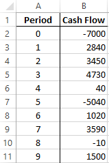
The amount of the initial investment is 7000. During the analyzed period there were two more investments – there are 5040 and 10.

Let`s go in the «Formula» tab. In the category «Financial» we find the IRR function. We fill in these arguments.

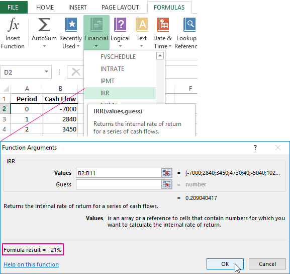
The values – is the range with the sums of cash flows, for which it is necessary to calculate the internal rate of return. We are omitting the assumption now.

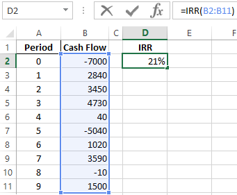
The required IRR (internal rate of return) of the analyzed project – is 0.209040416569432. If we transfer the decimal expression of the value in percentage, then we get the rate of 21%.

In our example, the calculation of the IRR is carried out for annual flows. If you need to find the IRR for monthly flows in just a few years, it’s better to enter the «Assumption» argument. The program can not cope with the calculation for 20 attempts – the error #NUMBER! will appear.

One more indicator of the efficiency of the investment project is NPV (the net discounted income). NPV and IRR are linked: the IRR defines the discount rate at which NPV = 0 (that is, the project costs are equal to the revenues).

For calculation NPV in Excel, the =NPV() function is applied. To find the internal rate of return using the graphical method, you need to build the change schedule in NPV. To do this, in the formula for calculating NPV we will substitute to the different values for discount rates.

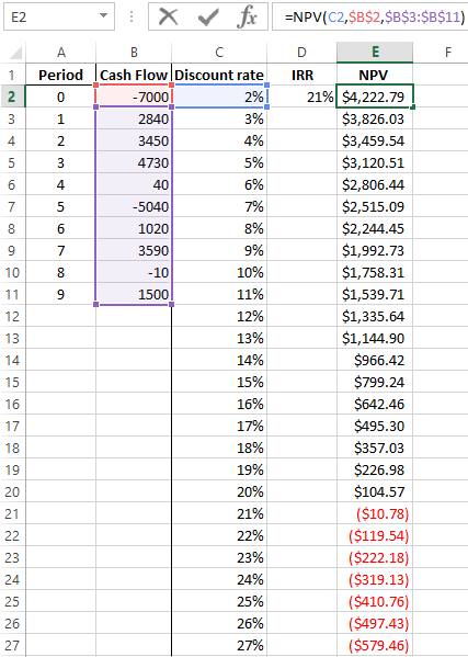
On the grounds of the obtained data, we plot the schedule change in NPV.

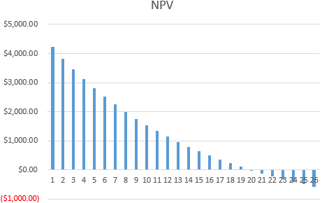
The intersection of the graph with the X axis (when the project’s net present value of income is zero) will give us the IRR index for this project. The graphical method showed the result, that is similar to found in Excel.

How to use the IRR indicator:

If the IRR value of the project is higher than the cost of capital for the enterprise, you must accept this investment project.

That is, if the loan rate is less than the internal rate of profitability, then borrowed funds will bring profit. Since in the implementation of the project we will get a higher percentage of income, than the amount of capital will be higher.

We return to our example now and suppose, that for the launch of the project a loan was taken in the bank at 15% per annum. The calculation showed that the internal rate of return was 20. 9%. You can earn on this project.

Источник

How to Calculate Internal Rate of Return (IRR) in Excel

What Is the Internal Rate of Return (IRR)?

The internal rate of return (IRR) is the discount rate providing a net value of zero for a future series of cash flows. Both the IRR and net present value (NPV) are used when selecting investments based on their returns.

Excel has three functions for calculating the internal rate of return that include Internal Rate of Return (IRR), Modified Internal Rate of Return (MIRR), and Internal Rate of Return with time periods (XIRR).

The IRR function calculates the internal rate of return for a series of cash flows, the MIRR function works with interest rates for borrowing and investing, and the XIRR function calculates a more accurate internal rate of return as it considers time periods.

Key Takeaways

• The internal rate of return (IRR) is the discount rate providing a net value of zero for a future series of cash flows.

• Excel has three functions for calculating the internal rate of return.

• When using different borrowing rates of reinvestment, a modified internal rate of return (MIRR) applies.

• The XIRR function accounts for different time periods.

How to Calculate IRR in Excel

What Is Net Present Value?

NPV is the difference between the present value of cash inflows and the present value of cash outflows over time.

The net present value of a project depends on the discount rate used. So when comparing two investment opportunities, the choice of the discount rate, which is often based on a degree of uncertainty, will have a considerable impact.

In the example below, using a 20% discount rate, investment #2 shows higher profitability than investment #1. When opting instead for a discount rate of 1%, investment #1 shows a return bigger than investment #2. Profitability often depends on the sequence and importance of the project’s cash flow and the discount rate applied to those cash flows.

How IRR and NPV Differ

The main difference between the IRR and NPV is that NPV is an actual amount while the IRR is the interest yield as a percentage expected from an investment.

Investors typically select projects with an IRR that is greater than the cost of capital. However, selecting projects based on maximizing the IRR as opposed to the NPV could result in suboptimal economic outcomes.

IRR represents the actual annual return on investment only when the project generates zero interim cash flows, or if those investments can be invested at the current IRR.

Calculating IRR in Excel

The IRR is the discount rate that can bring an investment’s NPV to zero. When the IRR has only one value, this criterion becomes more interesting when comparing the profitability of different investments.

In our example, the IRR of investment #1 is 48% and, for investment #2, the IRR is 80%. This means that in the case of investment #1, with an investment of $2,000 in 2013, the investment will yield an annual return of 48%. In the case of investment #2, with an investment of $1,000 in 2013, the yield will bring an annual return of 80%.

If no parameters are entered, Excel starts testing IRR values differently for the entered series of cash flows and stops as soon as a rate is selected that brings the NPV to zero. If Excel does not find any rate reducing the NPV to zero, it shows the error «#NUM.»

If the second parameter is not used and the investment has multiple IRR values, we will not notice because Excel will only display the first rate it finds that brings the NPV to zero.

In the image below, for investment #1, Excel does not find the NPV rate reduced to zero, so we have no IRR.

The image below also shows investment #2. If the second parameter is not used in the function, Excel will find an IRR of -10%. On the other hand, if the second parameter is used (i.e., = IRR ($ C $ 6: $ F $ 6, C12)), there are two IRRs rendered for this investment, which are -10% and 216%.

If the cash flow sequence has only a single cash component with one sign change (from + to — or — to +), the investment will have a unique IRR. However, most investments begin with a negative flow and a series of positive flows as the first investments come in. Profits then, hopefully, subside, as was the case in our first example.

In the image below, we calculate the IRR. To do this, we simply use the Excel IRR function:

Calculating MIRR in Excel

When a company uses different borrowing rates of reinvestment, the modified internal rate of return (MIRR) applies.

In the image below, we calculate the IRR of the investment as in the previous example but taking into account that the company will borrow money to plow back into the investment (negative cash flows) at a rate different from the rate at which it will reinvest the money earned (positive cash flow). The range C5 to E5 represents the investment’s cash flow range, and cells D10 and D11 represent the rate on corporate bonds and the rate on investments.

The image below shows the formula behind the Excel MIRR. We calculate the MIRR found in the previous example with the MIRR as its actual definition. This yields the same result: 56.98%.

Calculating XIRR in Excel

The XIRR function takes into consideration different periods. To use this function, Excel requires both the cash flow amounts as well as the dates on which those cash flows are paid.

In the example below, the cash flows are not disbursed at the same time each year – as is the case in the above examples. Rather, they are happening at different periods. We use the XIRR function below to solve this calculation. We first select the cash flow range (C5 to E5) and then select the range of dates on which the cash flows are realized (C32 to E32).

For investments with cash flows received or cashed at different moments in time for a firm that has different borrowing rates and reinvestments, Excel does not provide functions that can be applied to these situations although they are probably more likely to occur.

Источник

How to use Excel IRR function to calculate internal rate of return

by Svetlana Cheusheva, updated on March 15, 2023

This tutorial explains the syntax of the Excel IRR function and shows how to use an IRR formula to calculate the internal rate of return for a series of annual or monthly cash flows.

IRR in Excel is one of the financial functions for calculating the internal rate of return, which is frequently used in capital budgeting to judge projected returns on investments.

IRR function in Excel

The Excel IRR function returns the internal rate of return for a series of periodic cash flows represented by positive and negative numbers.

In all calculations, it’s implicitly assumed that:

• There are equal time intervals between all cash flows.
• All cash flows occur at the end of a period.
• Profits generated by the project are reinvested at the internal rate of return.

The function is available in all versions of Excel for Office 365, Excel 2019, Excel 2016, Excel 2013, Excel 2010 and Excel 2007.

The syntax of the Excel IRR function is as follows:

• Values (required) – an array or a reference to a range of cells representing the series of cash flows for which you want to find the internal rate of return.
• Guess (optional) – your guess at what the internal rate of return might be. It should be provided as a percentage or corresponding decimal number. If omitted, the default value of 0.1 (10%) is used.

For example, to calculate IRR for cash flows in B2:B5, you’d use this formula:

For the result to display correctly, please make sure the Percentage format is set for the formula cell (usually Excel does this automatically).

As shown in the above screenshot, our Excel IRR formula returns 8.9%. Is this rate good or bad? Well, it depends on several factors.

Generally, a calculated internal rate of return is compared to a company’s weighted average cost of capital or hurdle rate. If the IRR is higher than the hurdle rate, the project is considered a good investment; if lower, the project should be rejected.

In our example, if it costs you 7% to borrow money, then an IRR of about 9% is fairly good. But if the cost of funds is, say 12%, then the IRR of 9% is not good enough.

In reality, there are many other factors that influence an investment decision such as the net present value, absolute return value, etc. For more information, please see IRR basics.

5 things you should know about Excel IRR function

To ensure that your IRR calculation in Excel is done correctly, please remember these simple facts:

1. The values argument must contain at least one positive value (representing income) and one negative value (representing outlay).
2. Only numbers in the values argument are processed; text, logical values, or empty cells are ignored.
3. The cash flows do not necessarily have to be even, but they must occur at regular intervals, for example monthly, quarterly or annually.
4. Because IRR in Excel interprets the order of cash flows based on the order of values, the values should be in chronological order.
5. In most situations, the guess argument is not really needed. However, if the IRR equation has more than one solution, the rate closest to the guess is returned. So, your formula produces an unexpected result or a #NUM! error, try a different guess.

Understanding IRR formula in Excel

Since the internal rate of return (IRR) is a discount rate that makes the net present value (NPV) of a given series of cash flows equal to zero, the IRR calculation relies on the traditional NPV formula:

• CF — cash flow
• i — period number
• n — periods total
• IRR — internal rate of return

Because of a specific nature of this formula, there is no way to calculate IRR other than through trial and error. Microsoft Excel also relies on this technique but does multiple iterations extremely quickly. Starting with the guess (if supplied) or the default 10%, the Excel IRR function cycles through the calculation until it finds the result accurate within 0.00001%. If after 20 iterations an accurate result is not found, the #NUM! error is returned.

To see how it works in practice, let’s perform this IRR calculation on a sample data set. For starters, we will try to guess what the internal rate of return might be (say 7%), and then work out the net present value.

Assuming B3 is the cash flow and A3 is the period number, the following formula gives us the present value (PV) of the future cash flow:

Then we copy the above formula to other cells and add up all the present values, including the initial investment:

And find out that at 7% we get the NPV of $37.90:

Obviously, our guess is wrong. Now, let’s do the same calculation based on the rate computed by the IRR function (around 8.9%). Yep, it does lead to a zero NPV:

Tip. To display the exact NPV value, choose to show more decimal places or apply the Scientific format. In this example, the NPV is exactly zero, which is a very rare case!

Using IRR function in Excel – formula examples

Now that you know the theoretical basis of IRR calculation in Excel, let’s make a couple of formulas to see how it works in practice.

Example 1. Calculate IRR for monthly cash flows

Assuming you have been running business for six months and now you want to figure out the rate of return for your cash flow.

Finding IRR in Excel is very straightforward:

1. Type the initial investment into some cell (B2 in our case). Since it’s an outgoing payment, it needs to be a negative number.
2. Type the subsequent cash flows into the cells under or to the right of the initial investment (B2:B8 in this example). This money has been coming in through sales, so we enter these as positive numbers.

Now, you are ready to calculate IRR for the project:

=IRR(B2:B8)

Note. In event of monthly cash flows, the IRR function produces a monthly rate of return. To get an annual rate of return for monthly cash flow, you can use the XIRR function.

Example 2: Use guess in Excel IRR formula

Optionally, you can put an expected internal rate of return, say 10 percent, in the guess argument:

As shown in the screenshot below, our guess does not have any impact on the result. But in some cases, changing the guess value may cause an IRR formula to return a different rate. For more information, please see Multiple IRRs.

Example 3. Find IRR to compare investments

In capital budgeting, IRR values are often used to compare investments and rank projects in terms of their potential profitability. This example demonstrates the technique in its simplest form.

Supposing you have three investment options and you are deciding which one to choose. The reasonably projected returns on the investments can help you make an informed decision. For this, enter the cash flow for each project in a separate column, and then calculate the internal rate of return for each project individually:

Formula for project 1:

Formula for project 2:

Formula for project 3:

=IRR(D2:D7)

Given that the company’s required rate of return is, say 9%, project 1 should be rejected because its IRR is only 7%.

The two other investments are acceptable because both can generate an IRR higher than the company’s hurdle rate. Which one would you choose?

At first sight, project 3 looks more preferable because it has the highest internal rate of return. However, its yearly cash flows are much lower than for project 2. In situation when a small investment has a very high rate of return, businesses often choose an investment with a lower percentage return but higher absolute (dollar) return value, which is project 2.

The conclusion is: the investment with the highest internal rate of return is usually preferred, but to make the best use of your funds you should evaluate other indicators as well.

Example 4. Calculate compound annual growth rate (CAGR)

Though the IRR function in Excel is designed for calculating the internal return rate, it can also be used for computing the compound growth rate. You will just have to reorganize your original data in this way:

• Keep the first value of the initial investment as a negative number and the ending value as a positive number.
• Replace the interim cash flow values with zeros.

When done, write a regular IRR formula and it will return the CAGR:

To make sure the result is correct, you can verify it with the commonly used formula for calculating CAGR:

(end_value/start_value)^(1/no. of periods) -1

As shown in the screenshot below, both formulas produce the same result:

IRR and NPV in Excel

The internal rate of return and the net present value are two closely related concepts, and it’s impossible to fully understand IRR without understanding NPV. The result of IRR is nothing else but the discount rate corresponding to a zero net present value.

The essential difference is that NPV is an absolute measure that reflects the dollar amount of value that could be gained or lost by undertaking a project, while IRR is the percentage rate of return expected from an investment.

Because of their different nature, IRR and NPV may «conflict» with each other — one project may have a higher NPV and the other a higher IRR. Whenever such a conflict arises, finance experts advise to favor the project with a higher net present value.

To better understand the relationship between IRR and NPV, please consider the following example. Let’s say, you have a project that requires an initial investment of $1,000 (cell B2) and a discount rate of 10% (cell E1). The project’s lifespan is five years and the expected cash inflows for each year are listed in cells B3:B7.

To find out how much the future cash flows are worth now, we need to compute the net present value of the project. For this, use the NPV function and subtract the initial investment from it (because the initial investment is a negative number, the addition operation is used):

A positive net present value indicates that our project is going to be profitable:

What discount rate will make the NPV equal to zero? The following IRR formula gives the answer:

To check this, take the above NPV formula and replace the discount rate (E1) with IRR (E4):

Or you can embed the IRR function directly into the rate argument of NPV:

=NPV(IRR(B2:B7),B3:B7)+B2

The screenshot above shows that the NPV value rounded to 2 decimal places indeed equals zero. If you are curious to know the exact number, set the Scientific format to the NPV cell or choose to show more decimal places:

As you can see, the result is well within the declared accuracy of 0.00001 percent, and we can say that the NPV is effectively 0.

Tip. If you do not entirely trust the result of IRR calculation in Excel, you can always check it by using the NPV function like shown above.

Excel IRR function not working

If you have run into some problem with IRR in Excel, the following tips might give you a clue for fixing it.

IRR formula returns a #NUM! error

A #NUM! error may be returned because of these reasons:

• The IRR function fails to find the result with up to 0.000001% accuracy on the 20th try.
• The supplied values range does not contain at least one negative and at least one positive cash flow.

Blank cells in the values array

In case no cash flow arises in one or more periods, you may end up with empty cells in the values range. And it is the source of problems because rows with empty cells are left out of Excel IRR calculation. To fix this, just enter zero values in all blank cells. Excel will now see the correct time intervals and compute the internal return rate correctly.

Multiple IRRs

In situation when a cashflow series changes from negative to positive or vice versa more than once, multiple IRRs can be found.

If the result of your formula is far from what you expected, check the guess value – in case the IRR equation can be solved with several rate values, the rate closest to the guess is returned.

• Assuming that you know what kind of return you are expecting from a certain investment, use your expectation as a guess.
• When you get more than one IRR for the same cash flow, choose the one closest to your company’s cost of capital as the «true» IRR.
• Use the MIRR function to avoid the problem of multiple IRRs.

Irregular cash flow intervals

The IRR function in Excel is designed to work with regular cash flow periods such as weekly, monthly, quarterly or annually. If your inflows and outflows occur at unequal intervals, IRR would still consider the intervals equal and return a wrong result. In this case, use the XIRR function instead of IRR.

Different borrowing and reinvestment rates

The IRR function implies that the project earnings (positive cash flows) are continuously reinvested at the internal rate of return. But in the real word, the rate at which you borrow money and the rate at which you reinvest the profits are often different. Luckily for us, Microsoft Excel has a special function to take care of this scenario – the MIRR function.

That’s how to do IRR in Excel. To have a closer look at the examples discussed in this tutorial, you are welcome to download our sample workbook to Using IRR function in Excel. I thank you for reading and hope to see you on our blog next week!

Источник