Sumproduct and if in excel

SUMPRODUCT IF Formula – Excel & Google Sheets

Download the example workbook

This tutorial will demonstrate how to calculate “sumproduct if”, returning the sum of the products of arrays or ranges based­­ on criteria.

SUMPRODUCT Function

The SUMPRODUCT Function is used to multiply arrays of numbers, summing the resultant array.

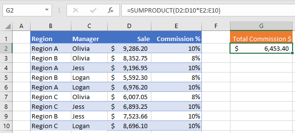
To create a “Sumproduct If”, we will use the SUMPRODUCT Function along with the IF Function in an array formula.

SUMPRODUCT IF

By combining SUMPRODUCT and IF in an array formula, we can essentially create a “SUMPRODUCT IF” that works similar to how the built-in SUMIF function works. Let’s walk through an example.

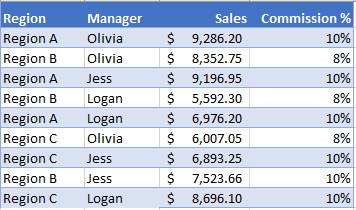
We have a list of sales by mangers in different regions with corresponding commission rates:

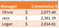
Supposed we are asked to calculate the commission amount for each manager like so:

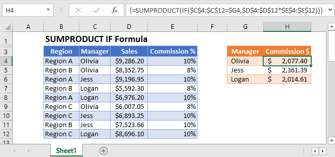
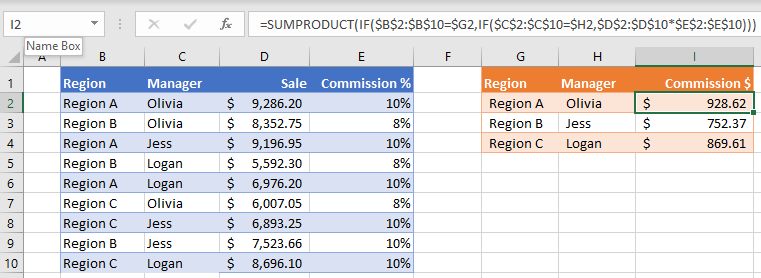
To accomplish this, we can nest an IF function with the manager as our criteria inside of the SUMPRODUCT function like so:

When using Excel 2019 and earlier, you must enter the formula by pressing CTRL + SHIFT + ENTER to get the curly brackets around the formula (see top image).

How does the formula work?

The formula works by evaluating each cell in our criteria range as TRUE or FALSE.

Calculating the total commission for Olivia:

Next, the IF Function replaces each value with FALSE if its condition is not met.

Now the SUMPRODUCT Function skips the FALSE values and sums the remaining values (2,077.40).

SUMPRODUCT IF with multiple criteria

To use SUMPRODUCT IF with multiple criteria (similar to how the built-in SUMIFS function works), simply nest more IF functions into the SUMPRODUCT function like so:

(CTRL + SHIFT + ENTER)

Another approach to SUMPRODUCT IF

Often in Excel, there are multiple ways to derive to the desired results. A different way to calculate “sumproduct if” is to include the criteria within the SUMPRODUCT function as an array using double unary like so:

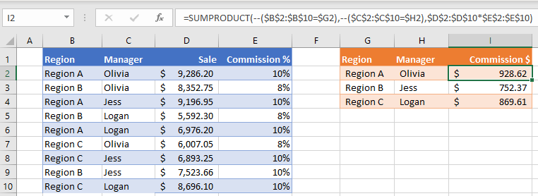
This method uses the double unary (–) to convert a TRUE FALSE array to zeros and ones. SUMPRODUCT then multiplies the converted criteria arrays together:

Tips and tricks:

• Where possible, always lock-reference (F4) your ranges and formula inputs to allow auto-filling.
• If you are using Excel 2019 or newer, you may enter the formula without Ctrl + Shift + Enter.

SUMPRODUCT IF in Google Sheets

The SUMPRODUCT IF Function works exactly the same in Google Sheets as in Excel, except you must use the ARRAYFORMULA Function instead of CTRL+SHIFT+ENTER to create the array formula.

Источник

SUMPRODUCT and IF function

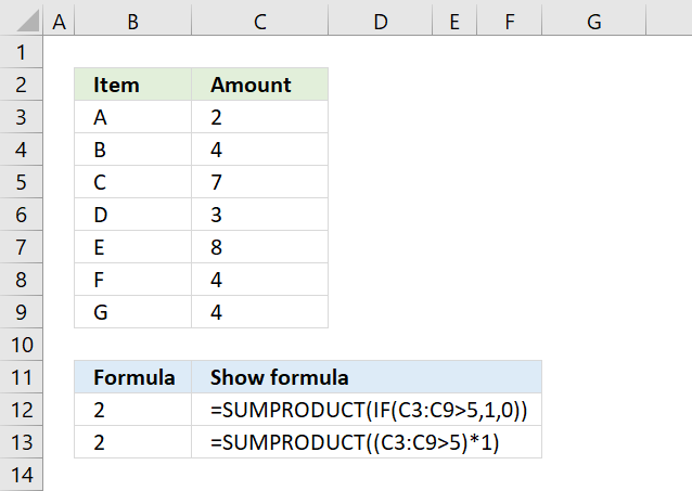
You don’t need to use the IF function in a SUMPRODUCT function, it is enough to use a logical expression. For example, the array formula above in cell B12 counts all cells in C3:C9 that are above 5 using an IF function.

Table of contents

1. How to simplify IF functions in the SUMPRODUCT function

The first argument in the IF function is a logical expression, use that in your SUMPRODUCT formula. The formula in B13 does the same thing as in B12.

You need to tell Excel the order of calculation, in other words, make sure you calculate C3:C9>5 before you multiply by 1. To do that use parentheses.

The larger than comparison operator compares each value in C3:C9 if larger than 5. It returns an array the same size as C3:C9 containing boolean values, TRUE or FALSE.

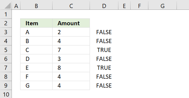
The picture above shows the array in column D, value 7 and 8 are larger than 5.

The SUMPRODUCT function can’t sum boolean values so multiply (using the asterisk *) the logical expression by 1 to convert the boolean values (TRUE and FALSE) to numbers (1 or 0).

The asterisk also has another advantage, you can enter the SUMPRODUCT formula as a regular formula.

1.1 Combine SUMPRODUCT and IF

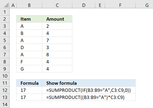
The picture above demonstrates an IF function that checks if a condition is met and if TRUE returns a value in a corresponding cell.

There is no need for the IF function in the above example, simply use the logical expression and multiply with the values you want to use, demonstrated in cell B13.

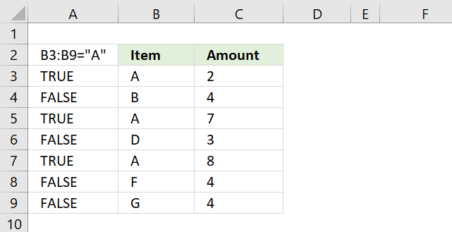
B3:B9=»A» returns displayed in column A in image above.

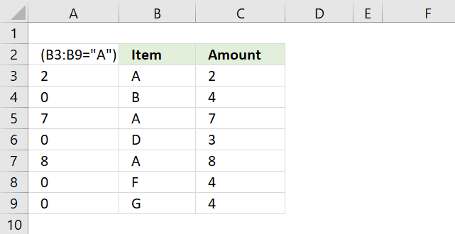
(B3:B9=»A»)*C3:C9 returns this array: <2;0;7;0;8;0;0>shown in column A.

Lastly, the SUMPRODUCT function sums all the numbers in the array returning 17 in cell B12.

2. SUMPRODUCT if greater than 0 (zero)

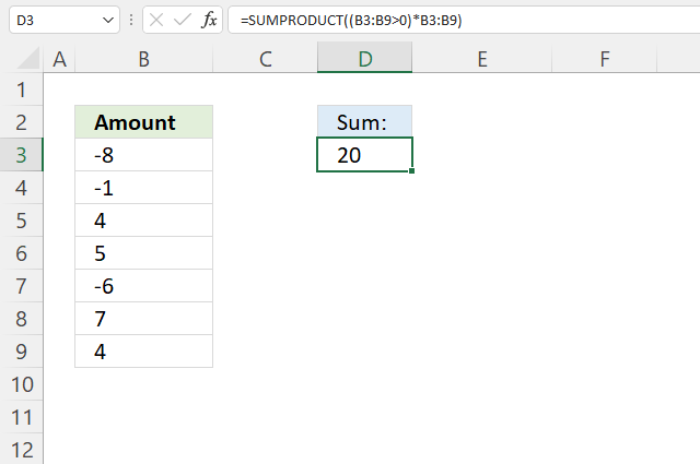
The formula in cell D3 adds numbers from B3:B9 if they are larger than 0 (zero) and returns a total.

Formula in cell D3:

2.1 Explaining formula

Step 1 — Check if values are larger than 0 (zero)

The larger than sign is a boolean operator that compares values to a condition, it returns TRUE or FALSE based on the outcome.

Step 2 — Multiply boolean values with numbers

The parentheses let you control the order of calculation, we must do the comparisons before we multiply.

The asterisk character lets you multiply a value with another value, in this case, with a boolean value.

TRUE is equal to 1 and FALSE is equal to 0 (zero), this will create the following outcomes:

TRUE * number = number
FALSE * number = 0 (zero)

Notice how all the negative numbers are converted to 0’s (zeros).

Step 3 — Add numbers and return total

The SUMPRODUCT function calculates the product of corresponding values and then returns the sum of each multiplication.

and returns 20 in cell D3.

3. SUMPRODUCT if between two dates

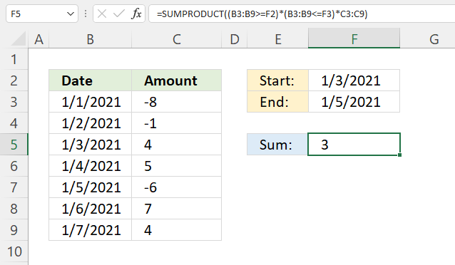
The SUMPRODUCT function shown in cell F5 calculates a total based on two dates. The example above demonstrates the start date in F2 and end date in F3, cells B5, B6, and B7 have dates that match the date range.

The corresponding numbers are in cells C5, C6, and C7. The total is calculated like this 4 + 5 — 6 equals 3.

Formula in cell f5:

Step 2 — Check which dates are equal to or earlier than the end date

The less than and the equal signs are boolean operators that compare values to a condition, it returns TRUE or FALSE based on the outcome.

B3:B9 =F2)*(B3:B9 =F2)*(B3:B9 =F2)*(B3:B9 F6))>0)*D3:D9)

5.1 Explaining formula

Step 1 — Evaluate condition

The equal sign compares value to value, however, not considering upper and lower cases. You need the EXACT function to do that.

Step 2 — Check if the number is larger than the condition

The larger than sign compares C3:C9 to number in F6, the result is a boolean value TRUE or FALSE.

Step 3 — Perform OR logic between arrays

The plus sign adds value to value, this applies OR logic between the arrays.

TRUE + TRUE = 1
TRUE + FALSE = 1
FALSE + TRUE = 1
FALSE + FALSE = 0 (zero)

This means that at least one condition must be met.

In Excel, any other number than 0 (zero) is considered to be TRUE even negative numbers. FALSE is 0 (zero).

Источник

SUMPRODUCT with IF

Related functions

Summary

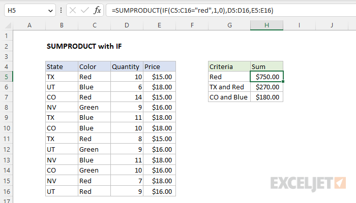
To create a conditional sum with the SUMPRODUCT function you can use the IF function or use Boolean logic. In the example shown, the formula in H5 is:

The result is $750, the total value of items with a color of «Red» in the data as shown. Note that SUMPRODUCT is not case-sensitive. Using the IF function inside SUMPRODUCT makes this into an array formula that must be entered with control + shift + enter in Legacy Excel. See below for an alternative Boolean syntax that does not need special handling.

Generic formula

Explanation

In this example, the goal is to calculate a conditional sum with the SUMPRODUCT function to match the criteria shown in G5:G7. One way to do this is to use the IF function directly inside of SUMPRODUCT. Another more common alternative is to use Boolean logic to apply criteria. Both approaches are explained below.

Basic SUMPRODUCT

The SUMPRODUCT function multiplies ranges or arrays together and returns the sum of products. The classic SUMPRODUCT problem multiplies two ranges together and sums the product directly without a helper column. For example, in the worksheet above, we have Quantity and Price, but no line item total. You can use SUMPRODUCT to get the total value of all records in the data like this:

In the worksheet shown, the result is $1,882, the sum of all quantities in D5:D16 multiplied by all prices in E5:E16. This formula works nicely. However, it’s not obvious how to calculate a conditional sum with SUMPRODUCT. For example, how can you calculate the value of all records where the color is «Red»? One option is to use the IF function directly, as explained in the next section.

SUMPRODUCT + IF function

One way to apply conditions with the SUMPRODUCT function is to use the IF function directly. This is the approach seen in the worksheet shown, where the formula in cell H5 is:

In this configuration, SUMPRODUCT has been given three arguments, array1, array2, and array3. Note that array2 holds Quantity and array3 holds Price. It is array1 that applies the conditional logic with the IF function like this:

Notice we are using 1 and 0 for the value_if_true and value_if_false arguments instead of the default TRUE and FALSE values. We do this because we want a numeric result, for reasons that become clear below. Because there are 12 values in the range C5:C16, IF returns an array with 12 results like this:

In this array, 1s indicate records where the color is «Red» and 0s indicate other colors. Dropping this array back into the SUMPRODUCT function, we have:

Now you can see how the logic works. The Boolean values that make up array1 act like a filter when the arrays are multiplied together. After multiplication, there is just a single array like this:

Note that the value of records where the color is not «Red» have been «zeroed out». The final result returned by SUMPRODUCT is $750. Additional conditions can be added with additional IF statements. To calculate a total for Color = «Red» and State = «TX», you can use the IF function twice like this:

The result is $270, as you can see in cell H6. The formula in cell H7 calculates a total for color = «Blue» and State = «CO» like this:

Although this formula works fine, one consequence of using the IF function inside of SUMPRODUCT is that it makes this into an array formula that must be entered with control + shift + enter in older versions of Excel that do not support dynamic array formulas. This is a bit unexpected, because one of SUMPRODUCT’s key strengths is the ability to handle array operations natively, but the IF function defeats this feature. The traditional solution to this problem is to switch to Boolean logic, as explained below.

SUMPRODUCT + Boolean logic

An alternative to using the IF function directly inside of SUMPRODUCT is to use Boolean logic. For example, to calculate the total value of records where the color is «Red», you can use a formula like this:

This example illustrates one of the key strengths of the SUMPRODUCT function – the ability to handle array operations natively. Inside SUMPRODUCT, the first array is a logical expression to filter on the color «red»:

SUMPRODUCT is not case-sensitive, so «red» will match «red», «Red», and «RED». Because there are 12 values in the range C5:C16, this expression returns an array with 12 results like this:

The double negative (—) then converts the TRUE and FALSE values to 1s and zeros:

Back in SUMPRODUCT, we now have:

Notice this is the same result we had with the IF function example above. As before, array1 acts like a filter when the arrays are multiplied together. After multiplication, there is just a single array like this:

All values associated with colors that are not «Red» have been «zeroed out», and the final result is $750. As with the IF function, the same pattern can be repeated to add more conditions. To calculate a total for Color = «Red» and State = «TX», you can use a formula like this:

To calculate a total for color = «Blue» and State = «CO», the formula is:

Simplifying with a single array

Excel pros will often simplify the syntax inside SUMPRODUCT by placing the conditional logic into a single argument like this

One advantage of this approach is that the math operation in array1 automatically coerces TRUE and FALSE into 1s and 0s, so we don’t need a double negative (—). Another advantage is that the math operation can be changed to apply a different type of logic. Instead of multiplication (*), which corresponds to AND logic in Boolean algebra, you can use addition (+), which corresponds to OR logic. For example, to sum the value of all records that are either «Red» or «Blue», you could use a formula like this:

As you can see, using Boolean logic with SUMPRODUCT is a flexible alternative to using the IF function, and it offers a major advantage: the formula will work fine in Legacy Excel, with no need to enter as an array formula with control + shift + enter.

Источник