- Relative and Absolute Cell References in MS Excel
- Relative Reference
- Absolute Reference
- Address Function in Excel
- Address Function in Excel
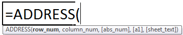
- Syntax of the ADDRESS Function
- How to Use the Address Function in Excel? (With Example)
- How to Use the INDIRECT Function to Pass the Address?
- Frequently Asked Questions
- Key Takeaways
- Recommended Articles
- Absolute, Relative, and Mixed Cell References in Excel
- What are Relative Cell References in Excel?
- When to Use Relative Cell References in Excel?
- What are Absolute Cell References in Excel?
- What does the Dollar ($) sign do?
- When to Use Absolute Cell References in Excel?
- What are Mixed Cell References in Excel?
- How to Change the Reference from Relative to Absolute (or Mixed)?
Relative and Absolute Cell References in MS Excel
Cell reference is the address or name of a cell or a range of cells. It is the combination of column name and row number. It helps the software to identify the cell from where the data/value is to be used in the formula. We can reference the cell of other worksheets and also of other programs.
- Referencing the cell of other worksheets is known as External referencing.
- Referencing the cell of other programs is known as Remote referencing.
There are two types of cell references in Excel:
- Relative reference
- Absolute reference
Relative Reference
Relative reference is the default cell reference in Excel. It is simply the combination of column name and row number without any dollar ($) sign. When you copy the formula from one cell to another the relative cell address changes depending on the relative position of column and row. C1, D2, E4, etc are examples of relative cell references. Relative references are used when we want to perform a similar operation on multiple cells and the formula must change according to the relative address of column and row.
For example, We want to add the marks of two subjects entered in column A and column B and display the result in column C. Here, we will use relative reference so that the same rows of column’s A and B are added.
Steps to Use Relative Reference:
Step 1: We write the formula in any cell and press enter so that it is calculated. In this example, we write the formula(= B2 + A2) in cell C2 and press enter to calculate the formula.
Step 2: Now click on the Fill handle at the corner of cell which contains the formula(C2).

Step 3: Drag the Fill handle up to the cells you want to fill. In our example, we will drag it till cell C10.
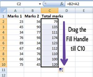
Step 4: Now we can see that the addition operation is performed between the cell A2 and B2, A3 and B3 and so on.
Step 5: You can double-click on any cell to check that the operation is performed in between which cells.
Thus, in the above example, we see that the relative address of cell A2 changes to A3, A4, and so on, similarly the relative address changes for column B, depending on the relative position of the row.
Absolute Reference
Absolute reference is the cell reference in which the row and column are made constant by adding the dollar ($) sign before the column name and row number. The absolute reference does not change as you copy the formula from one cell to other. If either the row or the column is made constant then it is known as a mixed reference. You can also press the F4 key to make any cell reference constant. $A$1, $B$3 are examples of absolute cell reference.
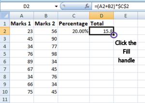
For example, We want to multiply the sum of marks of two subjects, entered in column A and column B, with the percentage entered in cell C2 and display the result in column D. Here, we will use absolute reference so that the address of cell C2 remains constant and does not change with the relative position of column and rows.
Steps to Use Absolute Reference:
Step 1: We write the formula in any cell and press enter so that it is calculated. In this example, we write the formula(=(A2+B2)*$C$2) in cell D2 and press enter to calculate the formula.
Step 2: Now click on the Fill handle at the corner of cell which contains the formula(D2).
Step 3: Drag the Fill handle up to the cells you want to fill. In our example, we will drag it till cell D10.
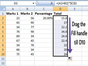
Step 4: Now we can see that the percentage is calculated in column D.
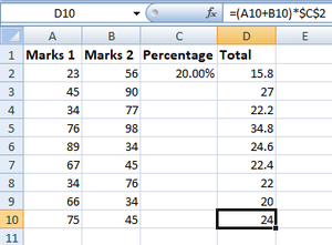
Step 5: You can double-click on any cell to check that the operation is performed in between which cells, and we see that the address of cell C2 does not change.
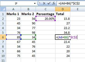
Thus, in the above example we see that the address of cell C2 is not changed whereas the address of column A and B changes with the relative position of the row and column, this happened because we used the absolute address of the cell C2.
Address Function in Excel


Address Function in Excel
The ADDRESS function returns the absolute address of the cell based on a specified row and column number. The cell address is returned as a text string. For example, “=ADDRESS(1,2)” returns “$B$1.” An inbuilt function of Excel, it is categorized under the lookup and reference functions.
Table of contents
Syntax of the ADDRESS Function
The syntax is stated as follows:
You are free to use this image on your website, templates, etc., Please provide us with an attribution link How to Provide Attribution? Article Link to be Hyperlinked
For eg:
Source: Address Function in Excel (wallstreetmojo.com)
The function accepts the following mandatory arguments:
- Row_Num: This is the row number used in the cell reference. The “row_num=1” represents row 1.
- Column_Num: This is the column number used in the cell reference. The “column_num= 2” represents column B.
The function accepts the following optional arguments:
- Abs_num (absolute number): This is the type of cell referenceCell ReferenceCell reference in excel is referring the other cells to a cell to use its values or properties. For instance, if we have data in cell A2 and want to use that in cell A1, use =A2 in cell A1, and this will copy the A2 value in A1.read more –absolute or relative. If this parameter is omitted, the default value is set at 1 (absolute). It can have any of the following values depending on the requirement:
| Abs_num | Explanation |
| 1 | Absolute referenceAbsolute ReferenceAbsolute reference in excel is a type of cell reference in which the cells being referred to do not change, as they did in relative reference. By pressing f4, we can create a formula for absolute referencing.read more like “$A$1” |
| 2 | Relative column, absolute row like “A$1” |
| 3 | Absolute column, relative row like “$A1” |
| 4 | Relative referenceRelative ReferenceIn Excel, relative references are a type of cell reference that changes when the same formula is copied to different cells or worksheets. Let’s say we have =B1+C1 in cell A1, and we copy this formula to cell B2 and it becomes C2+D2.read more like “A1” |
- A1: This is the reference style used. It can be either “A1” (1 or true) or “R1C1” (0 or false). If this parameter is omitted, the default style is “A1.”
- Sheet_text: This is the name of the sheet used in the cell address. If this parameter is omitted, no worksheet name is used.
How to Use the Address Function in Excel? (With Example)
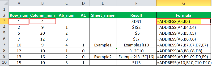
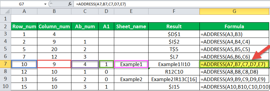
Let us consider the various possible outcomes of the ADDRESS function, as shown in the succeeding image.
The observations of a few rows are explained as follows:
1. The Third Row
- The “row=1” and “column=4.”
- The formula is “=ADDRESS(1,4).”
- By default, the parameters “absolute number” and “reference type” are set at 1.
- The result is an absolute address with an absolute row and an absolute column, i.e., “$D$1.”
- The “$D” signifies the absolute column “4” and “$1” signifies the absolute row “1.”
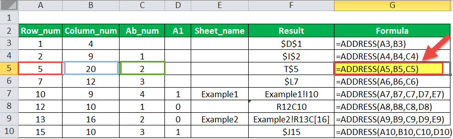
2. The Fifth Row
- The “row=5,” “column=20,” and “abs_num=2.”
- The ADDRESS formula can be rewritten in a simpler form as “=ADDRESS(5,20,2).”
- The reference style is set at 1 (true) when it has not been defined explicitly.
- The result is “T$5,” which has an absolute row ($5) and a relative column (T).
3. The Seventh Row
- We pass all the arguments of the ADDRESS function, including the optional ones.
- The “row=10,” “column=9,” “abs_num=4,” “A1=1,” and “sheet_name=Example1.”
- The address formula can be rewritten in a simpler form as “=ADDRESS(10,9,4,1,”Example1″).”
- The result is “Example1!I10.”
- Since the “absolute number” parameter is set at 4, the result is a relative reference (“I10”).
How to Use the INDIRECT Function to Pass the Address?
The reference of a cell can be derived with the help of the ADDRESS function. However, if we are interested in obtaining the value stored in the Excel address of cells, we use the INDIRECT function INDIRECT Function The INDIRECT excel function is used to indirectly refer to cells, cell ranges, worksheets, and workbooks. read more . With this function, we can get the actual value through reference.
Syntax of the INDIRECT Function
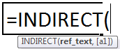
The function accepts the following arguments:
- Ref_text: This is the cell reference supplied in the form of a text string.
- A1: This is a logical value that specifies the style of reference. It can be either “A1” (true or omitted) or “R1C1” (false).
The first argument is mandatory, while the second is optional.
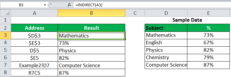
Let us consider an example.
The data is given in the following image. We want to find the value of the cell reference passed in the INDIRECT function.
In the first observation, the “ADDRESS=$D$3.” We rewrite the function as “=INDIRECT(A3).”
In cell D3, under the sample data, the value is “Mathematics.” This is the same as the result of the INDIRECT function in cell B3.
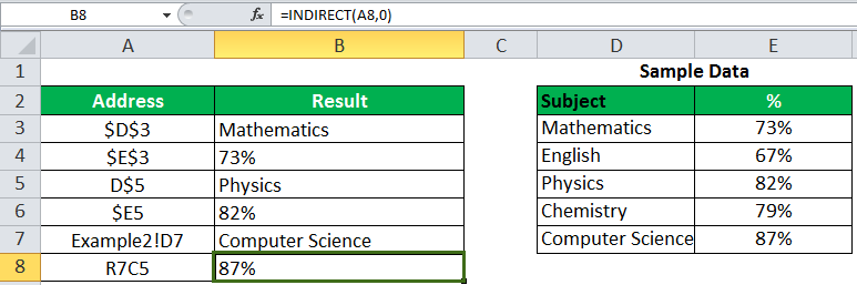
Let us consider another example in which the reference style is R7C5.
Here, we must set the “ref_type” to “false” (0), so that the INDIRECT function can read the reference style.
The output of “=INDIRECT(A8,0)” is 87%.
Frequently Asked Questions
The uses of the function are listed as follows:
– It is used to address the first or the last cell in a range.
– It helps convert a column number to a letter and vice versa.
– It is used to construct a cell reference within a formula.
– It helps find the cell value from the row and column number.
– It returns the address of the cell with the highest value.
The formula to return the full address of a named range is stated as follows:
“=ADDRESS(ROW(range), COLUMN(range)) & “:” & ADDRESS(ROW(range) + ROWS(range)-1, COLUMN(range) + COLUMNS(range)-1)”
“Range” is the named range whose address is required.
If the range address is required as a relative reference, the “abs_num” argument is set at 4. The formula can be rewritten as follows:
“=ADDRESS(ROW(range), COLUMN(range), 4) & “:” & ADDRESS(ROW(range) + ROWS(range)-1, COLUMN(range) + COLUMNS(range)-1, 4)”
Key Takeaways
- The ADDRESS function creates a cell address from a given row and column number.
- The syntax of the ADDRESS function is–“ADDRESS(row_num, column_num, [abs_num], [a1], [sheet_text]).”
- The “row_num” and “column_num” are mandatory arguments, while “abs_num,” “A1,” and “sheet_text” are optional arguments.
- The “abs_num” parameter can be set as follows:
- 1 or omitted–Absolute reference
- 2–Absolute row, relative column
- 3–Relative row, absolute column
- 4–Relative reference
- The reference style can be set at either “A1” (1 or true) or “R1C1” (0 or false).
- The default reference style is “A1.”
- The INDIRECT function helps obtain the value stored in the Excel address of cells. The syntax of the INDIRECT function is–“INDIRECT(ref_text, [a1]).”
Recommended Articles
This has been a guide to Address Excel Function. Here we discuss how to use the Address Formula in Excel along with step by step examples and downloadable Excel templates.`
Absolute, Relative, and Mixed Cell References in Excel
A worksheet in Excel is made up of cells. These cells can be referenced by specifying the row value and the column value.
For example, A1 would refer to the first row (specified as 1) and the first column (specified as A). Similarly, B3 would be the third row and second column.
The power of Excel lies in the fact that you can use these cell references in other cells when creating formulas.
Now there are three kinds of cell references that you can use in Excel:
- Relative Cell References
- Absolute Cell References
- Mixed Cell References
Understanding these different types of cell references will help you work with formulas and save time (especially when copy-pasting formulas).
This Tutorial Covers:
What are Relative Cell References in Excel?
Let me take a simple example to explain the concept of relative cell references in Excel.
Suppose I have a data set shown below:
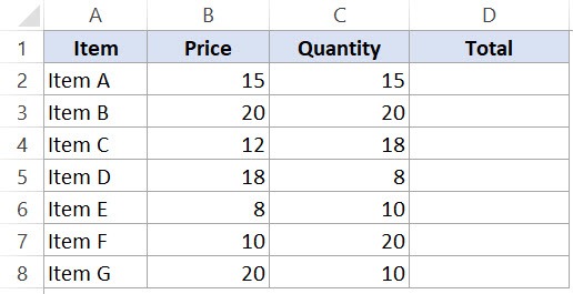
To calculate the total for each item, we need to multiply the price of each item with the quantity of that item.
For the first item, the formula in cell D2 would be B2* C2 (as shown below):
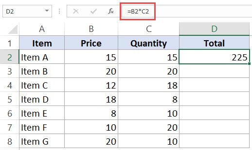
Now, instead of entering the formula for all the cells one by one, you can simply copy cell D2 and paste it into all the other cells (D3:D8). When you do it, you will notice that the cell reference automatically adjusts to refer to the corresponding row. For example, the formula in cell D3 becomes B3*C3 and the formula in D4 becomes B4*C4.
These cell references that adjust itself when the cell is copied are called relative cell references in Excel.
When to Use Relative Cell References in Excel?
Relative cell references are useful when you have to create a formula for a range of cells and the formula needs to refer to a relative cell reference.
In such cases, you can create the formula for one cell and copy-paste it into all cells.
What are Absolute Cell References in Excel?
Unlike relative cell references, absolute cell references don’t change when you copy the formula to other cells.
For example, suppose you have the data set as shown below where you have to calculate the commission for each item’s total sales.
The commission is 20% and is listed in cell G1.
![]()
To get the commission amount for each item sale, use the following formula in cell E2 and copy for all cells:
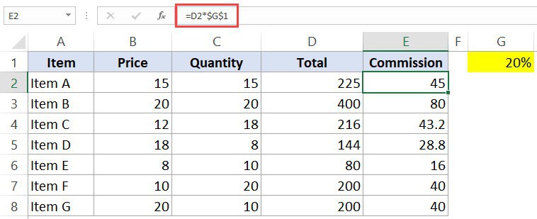
Note that there are two dollar signs ($) in the cell reference that has the commission – $G$2.
What does the Dollar ($) sign do?
A dollar symbol, when added in front of the row and column number, makes it absolute (i.e., stops the row and column number from changing when copied to other cells).
For example, in the above case, when I copy the formula from cell E2 to E3, it changes from =D2*$G$1 to =D3*$G$1.
Note that while D2 changes to D3, $G$1 doesn’t change.
Since we have added a dollar symbol in front of ‘G’ and ‘1’ in G1, it wouldn’t let the cell reference change when it’s copied.
Hence this makes the cell reference absolute.
When to Use Absolute Cell References in Excel?
Absolute cell references are useful when you don’t want the cell reference to change as you copy formulas. This could be the case when you have a fixed value that you need to use in the formula (such as tax rate, commission rate, number of months, etc.)
While you can also hard code this value in the formula (i.e., use 20% instead of $G$2), having it in a cell and then using the cell reference allows you to change it at a future date.
For example, if your commission structure changes and you’re now paying out 25% instead of 20%, you can simply change the value in cell G2, and all the formulas would automatically update.
What are Mixed Cell References in Excel?
Mixed cell references are a bit more tricky than the absolute and relative cell references.
There can be two types of mixed cell references:
- The row is locked while the column changes when the formula is copied.
- The column is locked while the row changes when the formula is copied.
Let’s see how it works using an example.
Below is a data set where you need to calculate the three tiers of commission based on the percentage value in cell E2, F2, and G2.
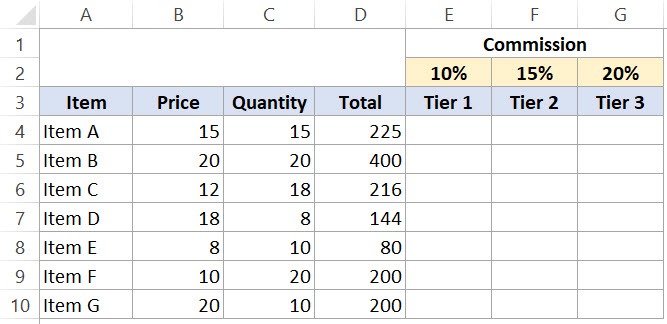
Now you can use the power of mixed reference to calculate all these commissions with just one formula.
Enter the below formula in cell E4 and copy for all cells.
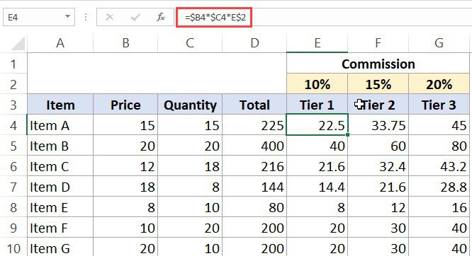
The above formula uses both kinds of mixed cell references (one where the row is locked and one where the column is locked).
Let’s analyze each cell reference and understand how it works:
- $B4 (and $C4) – In this reference, the dollar sign is right before the Column notation but not before the Row number. This means that when you copy the formula to the cells on the right, the reference will remain the same as the column is fixed. For example, if you copy the formula from E4 to F4, this reference would not change. However, when you copy it down, the row number would change as it is not locked.
- E$2 – In this reference, the dollar sign is right before the row number, and the Column notation has no dollar sign. This means that when you copy the formula down the cells, the reference will not change as the row number is locked. However, if you copy the formula to the right, the column alphabet would change as it’s not locked.
How to Change the Reference from Relative to Absolute (or Mixed)?
To change the reference from relative to absolute, you need to add the dollar sign before the column notation and the row number.
For example, A1 is a relative cell reference, and it would become absolute when you make it $A$1.
If you only have a couple of references to change, you may find it easy to change these references manually. So you can go to the formula bar and edit the formula (or select the cell, press F2, and then change it).
However, a faster way to do this is by using the keyboard shortcut – F4.
When you select a cell reference (in the formula bar or in the cell in edit mode) and press F4, it changes the reference.
Suppose you have the reference =A1 in a cell.
Here is what happens when you select the reference and press the F4 key.
- Press F4 key once: The cell reference changes from A1 to $A$1 (becomes ‘absolute’ from ‘relative’).
- Press F4 key two times: The cell reference changes from A1 to A$1 (changes to mixed reference where the row is locked).
- Press F4 key three times: The cell reference changes from A1 to $A1 (changes to mixed reference where the column is locked).
- Press F4 key four times: The cell reference becomes A1 again.
You May Also Like the Following Excel Tutorials: